Localizing oscillatory sources using beamformer techniques
Contents
- Introduction
- Background
- Procedure
- Create the volume conduction model
- Visualizing the headmodel
- Processing of the MEG data
- Identify the time and frequency range of interest
- Plotting the effect of interest
- DICS beamforming
- Source Analysis: Contrast activity to another interval
- Summary and suggested further reading
Introduction
In this tutorial we will continue working on the "visual gammaband" dataset described in the time-frequency analysis tutorial. Below we will repeat short sections the analysis pipeline to select the trials and preprocess the data as described in the earlier tutorials: trigger based trial selection and visual artifact rejection.
In this tutorial you will learn about applying beamformer techniques in the frequency domain. You will learn how to compute appropriate time-frequency windows, a good-quality head model and lead field matrices, and we touch upon various options for contrasting the effect of interest against some control/baseline. Finally, you will be shown several options for plotting the results overlaid on a structural MRI.
It is expected that you understand the previous steps of preprocessing and filtering the sensor data. Some understanding of the options for computing the head model and forward lead field is also useful.
This tutorial will not cover the time-domain option for LCMV/SAM beamformers, nor for beamformers applied to evoked/averaged data (although see here for an LCMV example).
Background
In the Time-Frequency Analysis tutorial we identified strong oscillations over visual regions in the gamma band. The goal of this section is to identify the sources responsible for producing this oscillatory activity. We will apply a beamformer technique. This is a spatially adaptive filter, allowing us to estimate the amount of activity at any given location in the brain. The inverse filter is based on minimizing the source power (or variance) at a given location, subject to 'unit-gain constraint'. This latter part means that, if a source had power of amplitude 1 and was projected to the sensors by the lead field, the inverse filter applied to the sensors should then reconstruct power of amplitude 1 at that location. Beamforming assumes that sources in different parts of the brain are not temporally correlated.
The brain is divided in a regular three dimensional grid and the source strength for each grid point is computed. The method applied in this example is termed Dynamical Imaging of Coherent Sources (DICS) and the estimates are calculated in the frequency domain (Gross et al. 2001). Other beamformer methods rely on sources estimates calculated in the time domain, e.g. the Linearly Constrained Minimum Variance (LCMV) and Synthetic Aperture Magnetometry (SAM) methods (van Veen et al., 1997; Robinson and Cheyne, 1997). These methods produce a 3D spatial distribution of the power of the neuronal sources. This distribution is then overlaid on a structural image of the subject's brain. Furthermore, these distributions of source power can be subjected to statistical analysis. It is always ideal to contrast the activity of interest against some control/baseline activity. Options for this will be discussed below, but it is best to keep this in mind when designing your experiment from the start, rather than struggle to find a suitable control/baseline after data collection.
Procedure
The first section of this tutorial deals with processing the anatomical data and constructing the volume conduction model. For this, we will perform the following steps:
- Read the anatomical MRI and headshape with ft_read_mri and ft_read_headshape
- Align the anatomical MRI to the MEG coordinate system
- Construct a volume conduction model using ft_volumesegment and ft_prepare_headmodel
In the second part of this tutorial we will proceed with the functional data and actiually localize the sources of the gamma band activity:
- Read the MEG data into MATLAB using ft_definetrial and ft_preprocessing
- Compute the cross-spectral density matrix using the function ft_freqanalysis
- Compute the forward solution (lead field matrix) using ft_prepare_leadfield
- Compute a spatial filter and estimate the power of the sources using ft_sourceanalysis
- Visualize the results, by first interpolating the sources to the anatomical MRI using ft_sourceinterpolate and plotting this with ft_sourceplot.
filename = 'workshop_visual_sss.fif';

mrifile1 = '../MRI/dicom/00000001.dcm'; % you can read from dicom files
mrifile2 = '../MRI/daniel_t1.nii';      % reading from the nifti is faster than from the dicoms

mri = ft_read_mri(mrifile2);
We can visualize the anatomical MRI together with the x/y/z axes and origin using the ft_determine_coordsys function. Normally it is used to interactively determine the coordinate system, i.e. figure out whether x is towards the nose etc. Here we disable the interactive mode to just get the 3-D figure.
ft_determine_coordsys(mri, 'interactive', 'no');
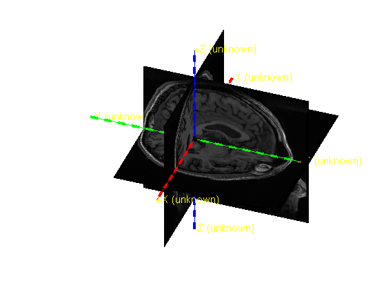
You can see that the origin is not at the appropriate location and that the axes do not intersect with the scalp surface at the fiducial locations.
The other piece of information that we have is the location of the fiducials and the headshape, which are both measured using a Polhemus 3-D tracker just prior to the MEG measurement. The headshape information is stored in the fiff file together with the MEG data
headshape = ft_read_headshape(filename);
	306 MEG channel locations transformed
Opening raw data file workshop_visual_sss.fif...
	Range : 7000 ... 994999  =      7.000 ...   994.999 secs
Ready.
HACK: To prevent an error further down in the code with the present version of FieldTrip (which does not like the single precision fiducial points), we convert these to double precision. This will of course be fixed in future GieldTrip releases.
headshape.fid.pnt = double(headshape.fid.pnt);
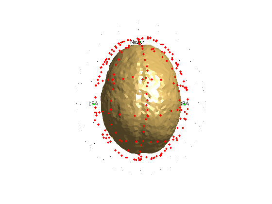
Also the headshape informatino can be plotted with the x/y/z axes and origin.
ft_determine_coordsys(headshape, 'interactive', 'no');
The positive x-axis is pointing towards the right
The positive y-axis is pointing towards anterior
The positive z-axis is pointing towards superior
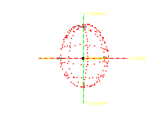
You see that in the headshape the axes pass through the Nasion, LPA and RPA fiducials.
We can align the surface of the anatomical MRI to the headshape with ft_volumerealign and the following code.
cfg = [];
cfg.method = 'headshape';
cfg.headshape = headshape; % or you can specify the filename
mri_realigned = ft_volumerealign(cfg, mri);
save mri_realigned.mat mri_realigned
INSTRUCTION: The piece of code above is not included in the flow of this tutorial due to layout limitations of the MATLAB publisher. You should execute it nevertheless!
The realignment consists of three steps: # the general orientation of the coordinate system is determined # a coarse interactive realignment between theadshape and MRI skin surface is interactively performed # the coregistration is refined using the iterative-closest-point algorithm, fitting the headshape to the MRI skin surface
In step 1 you should answer in the command window: y(es), r(ight), a(nterior), s(uperior), n(ot a landmark).
In step 2, you can rotate the figure and enter a translation. Along the y-axis you shoudl shift with approximately -25 mm, along the z-axis with 45 mm. After shifting the skin surface, you press the "quit" button.
Step 3 goes fully automatic.
After the realignment we can inspect the data structure:
load mri_realigned.mat

disp(mri_realigned)
              dim: [256 256 206]
          anatomy: [256x256x206 double]
              hdr: [1x1 struct]
        transform: [4x4 double]
             unit: 'mm'
    transformorig: [4x4 double]
         coordsys: 'neuromag'
              cfg: [1x1 struct]
Specifically interesting is to compare the original homogenous coordinate transformation matrix to the updated one:
disp(mri_realigned.transformorig)
   -0.9375         0         0  122.2365
         0   -0.9375         0  141.2485
         0         0    1.0000  -56.1470
         0         0         0    1.0000
disp(mri_realigned.transform)
   -0.9369    0.0009   -0.0358  128.6884
   -0.0078   -0.9175    0.2052  121.8768
   -0.0326    0.1926    0.9781  -81.2275
         0         0         0    1.0000
The "transform" matrix represents the rotations, scaling and translation that are aplied to the voxel indices (i.e. integers) to express the voxels in head coordinates and in milimeter.
The resulting realigned MRI is now expressed in Neuromag head coordinates, hence we can update the coordsys field from "unknown" to "neuromag".
mri_realigned.coordsys = 'neuromag';
INSTRUCTION: update the coordsys field, otherwise a piece of code further down will not work as expected!
Once more we use ft_determine_coordsys to look at the axes in relatino to the anatomical MRI.
ft_determine_coordsys(mri_realigned, 'interactive', 'no');
The positive x-axis is pointing towards the right
The positive y-axis is pointing towards anterior
The positive z-axis is pointing towards superior
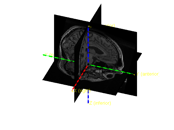
The axes are now in accordance with the anatomical landmarks.
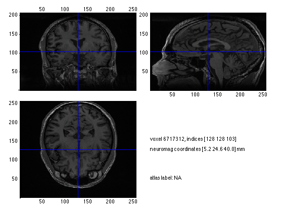
INSTRUCTION: Plot the anatomical MRI and check the location of the fiducials by clicking in the figure. Note the difference in voxel coordinates and head coordinates. See the code below:
cfg = [];
ft_sourceplot(cfg, mri_realigned);
the input is volume data with dimensions [256 256 206]
scaling anatomy to [0 1]
no functional parameter
no masking parameter
Warning: no colorbar possible without functional data

click left mouse button to reposition the cursor
click and hold right mouse button to update the position while moving the mouse
use the arrowkeys to navigate in the current axis
the call to "ft_sourceplot" took 1 seconds and required the additional allocation of an estimated 226 MB
After realigning, it can be desireable to reslice the anatomical MRI. This makes the axes of the voxels consistent with the axes of the head coordinate system.
cfg = [];
mri_resliced = ft_volumereslice(cfg, mri_realigned);
the input is volume data with dimensions [256 256 206]
reslicing from [256 256 206] to [256 256 256]
the input is volume data with dimensions [256 256 206]
the input is volume data with dimensions [256 256 256]
selecting subvolume of 68.9%
reslicing and interpolating anatomy
interpolating
interpolating 100.0%

the call to "ft_sourceinterpolate" took 53 seconds and required the additional allocation of an estimated 0 MB
the call to "ft_volumereslice" took 54 seconds and required the additional allocation of an estimated 0 MB
Having done the realignment and reslicing, it would be good to save the results.
save mri_resliced.mat mri_resliced
Create the volume conduction model
We proceed with segmenting the anatomical MRI to extract the brain compartment. Here FieldTrip makes use of the SPM segmentation functions (included in fieldtrip/external/spm8), and starts with a probabilistic segmentation of white matter, grey matter and CSF, which are subsequently combined in a single binary "brain" mask consistent with the inside of the skull.
cfg = [];
cfg.output = {'brain'}; % we need the brain, i.e. the inside of the skull
mri_segmented = ft_volumesegment(cfg, mri_resliced);

save mri_segmented.mat mri_segmented
the input is volume data with dimensions [256 256 256]
Warning: adding /Users/robert/matlab/fieldtrip/external/spm8 toolbox to your
Matlab path
Converting the coordinate system from neuromag to spm
Rescaling NIFTI: slope = 0.00342945, intercept = 0
Smoothing by 0 & 8mm..
Coarse Affine Registration..
Fine Affine Registration..
performing the segmentation on the specified volume
creating brainmask
smoothing brainmask with a 5-voxel FWHM kernel
thresholding brainmask at a relative threshold of 0.500
This step is quite timeconsuming, so you will probably want to press ctrl-c to abort it and read the results from file.
load mri_segmented
The voume conduction model we will be using is a realisting single-shell approximation to the inside of the skull.
cfg = [];
cfg.method = 'singleshell';
headmodel = ft_prepare_headmodel(cfg, mri_segmented);

save headmodel.mat headmodel
Warning: please specify cfg.method='projectmesh', 'iso2mesh' or 'isosurface'
Warning: using 'projectmesh' as default
triangulating the outer boundary of compartment 1 (brain) with 3000 vertices
the call to "ft_prepare_mesh" took 10 seconds and required the additional allocation of an estimated 19 MB
the call to "ft_prepare_headmodel" took 10 seconds and required the additional allocation of an estimated 20 MB
Visualizing the headmodel
We can plot everything together with some low-level FieldTrip functions from the fieldtrip/plotting directories. To get an overview of those functions, you can look at the help for the whole directory and the help of the individual functions
help plotting
Contents of plotting:

ft_plot_box                    - plots the outline of a box that is specified by its lower
ft_plot_dipole                 - makes a 3-D representation of a dipole using a small sphere
ft_plot_headshape              - visualizes the shape of a head from a variety of
ft_plot_lay                    - plots a two-dimensional layout
ft_plot_line                   - helper function for plotting a line, which can also be used in
ft_plot_matrix                 - visualizes a matrix as an image, similar to IMAGESC.
ft_plot_mesh                   - visualizes the information of a mesh contained in the first
ft_plot_montage                - makes a montage of a 3-D array by selecting slices at
ft_plot_ortho                  - plots a 3 orthographic cuts through a 3-D volume
ft_plot_sens                   - plots the position of the channels in the EEG or MEG sensor array
ft_plot_slice                  - cuts a 2-D slice from a 3-D volume and interpolates if needed
ft_plot_text                   - helper function for plotting text, which can also be used in
ft_plot_topo                   - interpolates and plots the 2-D spatial topography of the
...
help ft_plot_vol
  FT_PLOT_VOL visualizes the boundaries in the vol structure constituting the
  geometrical information of the forward model

  Use as
    hs = ft_plot_vol(vol, varargin)

  Graphic facilities are available for vertices, edges and faces. A list of
  the arguments is given below with the correspondent admitted choices.

      'facecolor'     [r g b] values or string, for example 'brain', 'cortex', 'skin', 'black', 'red', 'r'
      'vertexcolor'   [r g b] values or string, for example 'brain', 'cortex', 'skin', 'black', 'red', 'r'
      'edgecolor'     [r g b] values or string, for example 'brain', 'cortex', 'skin', 'black', 'red', 'r'
      'facealpha'     number between 0 and 1
      'faceindex'     true or false
      'vertexindex'   true or false
...
Let's also read the sensor positions and visualize them along with the rest.
sens = ft_read_sens(filename); % this reads sensor positions from the MEG data

figure
ft_plot_vol(headmodel, 'facecolor', 'skin', 'edgecolor', 'none')
ft_plot_headshape(headshape)
ft_plot_sens(sens)
camlight
alpha 0.5
	306 MEG channel locations transformed
Opening raw data file workshop_visual_sss.fif...
	Range : 7000 ... 994999  =      7.000 ...   994.999 secs
Ready.
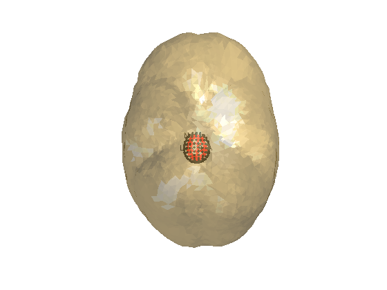
NOTE: This figure does not work out as expected. The FieldTrip low-level functions do not automatically deal with unit conversions, and the geometrical objects plotted here are a mixture of cm and mm.
disp(headmodel);
     bnd: [1x1 struct]
    type: 'singleshell'
    unit: 'mm'
     cfg: [1x1 struct]
disp(headshape);
         pnt: [204x3 double]
         fid: [1x1 struct]
       label: {1x204 cell}
    coordsys: 'neuromag'
        unit: 'cm'
disp(sens);
     balance: [1x1 struct]
     chanori: [306x3 double]
     chanpos: [306x3 double]
    chantype: {306x1 cell}
    chanunit: {306x1 cell}
     coilori: [510x3 double]
     coilpos: [510x3 double]
    coordsys: 'neuromag'
       label: {306x1 cell}
         tra: [306x510 double]
        type: 'neuromag306'
        unit: 'cm'
We can explicitly convert the units to a consistent representation using ft_convert_units
headmodel = ft_convert_units(headmodel, 'cm');

figure
ft_plot_vol(headmodel, 'facecolor', 'skin', 'edgecolor', 'none')
ft_plot_headshape(headshape)
ft_plot_sens(sens)
camlight
That looks much better! You can use the MATLAB rotate tool to visually inspect the relative locations of the inside of the skull (head model), the headshape points on the skin, and the location of the MEG channels.
Processing of the MEG data
cfg = [];
cfg.dataset   = filename;
cfg.trialfun  = 'trialfun_visual_stimulus';
cfg = ft_definetrial(cfg);

cfg.channel         = 'MEGGRAD';
cfg.baselinewindow  = [-inf 0];
cfg.demean          = 'yes';
data = ft_preprocessing(cfg);
evaluating trialfunction 'trialfun_visual_stimulus'
	306 MEG channel locations transformed
Opening raw data file workshop_visual_sss.fif...
	Range : 7000 ... 994999  =      7.000 ...   994.999 secs
Ready.
	306 MEG channel locations transformed
Opening raw data file workshop_visual_sss.fif...
	Range : 7000 ... 994999  =      7.000 ...   994.999 secs
Ready.
Reading 7000 ... 994999  =      7.000 ...   994.999 secs... [done]
found 1473 events
created 125 trials
the call to "ft_definetrial" took 27 seconds and required the additional allocation of an estimated 0 MB
	306 MEG channel locations transformed
Opening raw data file workshop_visual_sss.fif...
...
INSTRUCTION: Remove trials that have large variance from the raw data using ft_rejectvisual. Press "quit" once you are done removing bad trials.
cfg = [];
cfg.method = 'summary';
dataclean = ft_rejectvisual(cfg, data);
the input is raw data with 204 channels and 125 trials
Warning: correcting numerical inaccuracy in the time axes
showing a summary of the data for all channels and trials
computing metric [--------------------------------------------------------/]
112 trials marked as GOOD, 13 trials marked as BAD
204 channels marked as GOOD, 0 channels marked as BAD
the following trials were removed: 7, 12, 23, 24, 39, 50, 52, 60, 62, 74, 92, 101, 111
the call to "ft_rejectvisual" took 324 seconds and required the additional allocation of an estimated 19 MB
Identify the time and frequency range of interest
In the timefrequency tutorial you have seen that there is a sustained gamma-band effect following stimulus onset. We can reload the frequency decomposed data to have another look at it.
load visual_TFRmult

cfg = [];
TFRmult_cmb = ft_combineplanar(cfg, TFRmult);

cfg = [];
cfg.layout        = 'neuromag306cmb.lay';
cfg.baselinetype  = 'relchange';
cfg.baseline      = [-inf 0];
cfg.renderer      = 'painters'; % the default is OpenGL, which is faster, but it gives visual artifacts on some computers
cfg.colorbar      = 'yes';
cfg.zlim          = [-0.2 0.2];
figure
ft_multiplotTFR(cfg, TFRmult_cmb);
the input is freq data with 204 channels, 23 frequencybins and 43 timebins
the call to "ft_combineplanar" took 0 seconds and required the additional allocation of an estimated 3 MB
reading layout from file neuromag306cmb.lay
the call to "ft_prepare_layout" took 0 seconds and required the additional allocation of an estimated 1 MB
the input is freq data with 102 channels, 23 frequencybins and 43 timebins
the call to "ft_freqbaseline" took 0 seconds and required the additional allocation of an estimated 1 MB
Warning: (one of the) axis is/are not evenly spaced, but plots are made as if
axis are linear
the call to "ft_multiplotTFR" took 2 seconds and required the additional allocation of an estimated 4 MB
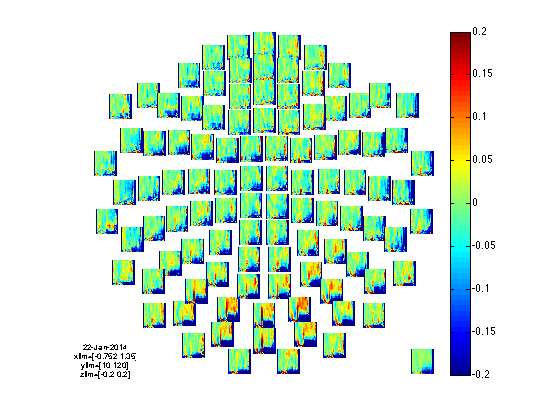
You can use the interactive feature to identify the occipital channels that show the effect the most. We can plot this in more detail and with better control over the plotting options using
cfg = [];
cfg.channel       = {'MEG1922+1923', 'MEG1932+1933', 'MEG2032+2033', 'MEG2042+2043', 'MEG2112+2113', 'MEG2322+2323', 'MEG2332+2333', 'MEG2342+2343', 'MEG2512+2513'};
cfg.layout        = 'neuromag306cmb.lay';
cfg.baselinetype  = 'relchange';
cfg.baseline      = [-inf 0];
cfg.colorbar      = 'yes';
cfg.zlim          = [-0.2 0.2]; % this will cause clipping for the lower frequeny-band effects
ft_singleplotTFR(cfg, TFRmult_cmb);
grid on
the input is freq data with 102 channels, 23 frequencybins and 43 timebins
the call to "ft_freqbaseline" took 0 seconds and required the additional allocation of an estimated 0 MB
the call to "ft_singleplotTFR" took 1 seconds and required the additional allocation of an estimated 0 MB
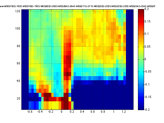
Based on this figure we select two intervals that are equally widein the baseline and stimulus window. Also relevant to note at this moment is that the frequency range of interest ranges from 60 all the way up to 120 Hz.
We already have the full data segments in memory. The frequency analysis is faster and can be more precisely controlled by taking a subselection of that data with ft_redefinetrial.
cfg = [];
cfg.toilim = [-0.400 0.000];
data_pre   = ft_redefinetrial(cfg, dataclean);

cfg.toilim = [ 0.250 0.650];
cfg.minlength = 'maxperlen'; % we don't want short fragments of data
data_post  = ft_redefinetrial(cfg, dataclean);
the input is raw data with 204 channels and 112 trials
Warning: correcting numerical inaccuracy in the time axes
removing 0 trials in which no data was selected
the call to "ft_redefinetrial" took 0 seconds and required the additional allocation of an estimated 68 MB
the input is raw data with 204 channels and 112 trials
Warning: correcting numerical inaccuracy in the time axes
removing 0 trials in which no data was selected
removing 7 trials that are too short
the call to "ft_redefinetrial" took 0 seconds and required the additional allocation of an estimated 69 MB
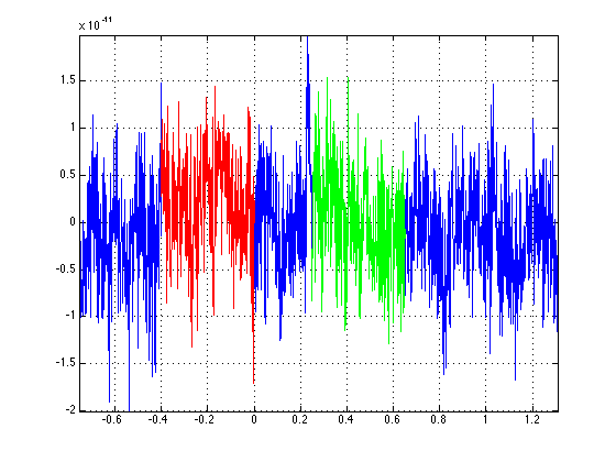
The following figure clarifies which sections of data we now have in data_pre and data_post. It plots channel 1 in trial 1 in blue for the original data, and red/green for the pre and post.
figure
plot(dataclean.time{1}, dataclean.trial{1}(1,:));
hold on
plot(data_pre.time{1}, data_pre.trial{1}(1,:), 'r');
plot(data_post.time{1}, data_post.trial{1}(1,:), 'g');
axis tight
grid on
However, we don't have an equal number of trials in data_pre and data_post.
disp(data_pre)
           hdr: [1x1 struct]
         label: {204x1 cell}
          time: {1x112 cell}
         trial: {1x112 cell}
       fsample: 1000
    sampleinfo: [112x2 double]
     trialinfo: [112x2 double]
          grad: [1x1 struct]
           cfg: [1x1 struct]
disp(data_post)
           hdr: [1x1 struct]
         label: {204x1 cell}
          time: {1x10⁵ cell}
         trial: {1x10⁵ cell}
       fsample: 1000
    sampleinfo: [105x2 double]
     trialinfo: [105x2 double]
          grad: [1x1 struct]
           cfg: [1x1 struct]
INSTRUCTION: explain why the number of trials differs. How can you find out which trials in data_pre belong to which trials in data_post?
cfg = [];
data_pre  = ft_rejectvisual(cfg, data_pre);
data_post = ft_rejectvisual(cfg, data_post);
the input is raw data with 204 channels and 112 trials
showing a summary of the data for all channels and trials
computing metric [---------------------------------------------------------]
104 trials marked as GOOD, 8 trials marked as BAD
204 channels marked as GOOD, 0 channels marked as BAD
the following trials were removed: 12, 49, 62, 82, 86, 98, 100, 106
the call to "ft_rejectvisual" took 7 seconds and required the additional allocation of an estimated 11 MB
the input is raw data with 204 channels and 105 trials
showing a summary of the data for all channels and trials
computing metric [--------------------------------------------------------/]
101 trials marked as GOOD, 4 trials marked as BAD
204 channels marked as GOOD, 0 channels marked as BAD
the following trials were removed: 15, 57, 77, 87
the call to "ft_rejectvisual" took 5 seconds and required the additional allocation of an estimated 5 MB
Since we have our time-windows of interest, we don't have to perform a time-resolved frequency analysis. Rather, we will use multitapers for the whole segment.
cfg = [];
cfg.method    = 'mtmfft';
cfg.output    = 'pow';    % we only need the power for now
cfg.taper     = 'dpss';
cfg.foi       = 5:5:150;
cfg.tapsmofrq = 10;       % we apply plenty of frequency smoothing
% cfg.tapsmofrq = 2;

freq_pre  = ft_freqanalysis(cfg, data_pre);
freq_post = ft_freqanalysis(cfg, data_post);
the input is raw data with 204 channels and 104 trials
processing trials
processing trial 104/104 nfft: 401 samples, datalength: 401 samples, 7 tapers

the call to "ft_freqanalysis" took 5 seconds and required the additional allocation of an estimated 3 MB
the input is raw data with 204 channels and 101 trials
processing trials
processing trial 101/101 nfft: 401 samples, datalength: 401 samples, 7 tapers

the call to "ft_freqanalysis" took 4 seconds and required the additional allocation of an estimated 1 MB
disp(freq_post)
        label: {204x1 cell}
       dimord: 'chan_freq'
         freq: [1x30 double]
    powspctrm: [204x30 double]
         grad: [1x1 struct]
          cfg: [1x1 struct]
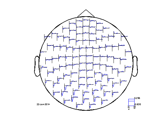
The power spectra can be plotted using ft_multiplotER, the same function that is used for plotting ERFs.
cfg = [];
freq_precmb  = ft_combineplanar(cfg, freq_pre);
freq_postcmb = ft_combineplanar(cfg, freq_post);

cfg = [];
cfg.layout        = 'neuromag306cmb.lay';
ft_multiplotER(cfg, freq_pre_cmb, freq_post_cmb);
the input is freq data with 204 channels, 30 frequencybins and no timebins
the call to "ft_combineplanar" took 0 seconds and required the additional allocation of an estimated 1 MB
the input is freq data with 204 channels, 30 frequencybins and no timebins
the call to "ft_combineplanar" took 0 seconds and required the additional allocation of an estimated 1 MB
selection powspctrm along dimension 1
selection powspctrm along dimension 1
reading layout from file neuromag306cmb.lay
the call to "ft_prepare_layout" took 0 seconds and required the additional allocation of an estimated 0 MB
the call to "ft_multiplotER" took 2 seconds and required the additional allocation of an estimated 3 MB
It is not directly obvious in this plot where the interesting effects are due to the spectral leakage of the low frequency activity, smearing the depression of the alpha and beta activity. The feature of interest is the small (approximately 10%) increase of gamma-band power in the range of 70-90 Hz.
Plotting the effect of interest
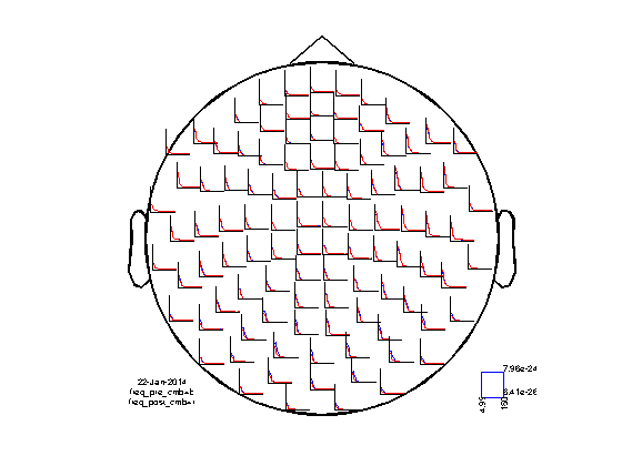
Similar to the visualization of the TFR relative to the baseline period, we can look at the powerspectrum of the post- relative to the pre-stimuls window.
freq_ratiocmb = freq_postcmb;
freq_ratiocmb.powspctrm = freq_postcmb.powspctrm ./ freq_precmb.powspctrm - 1;

cfg = [];
cfg.layout      = 'neuromag306cmb.lay';
cfg.parameter   = 'powspctrm';
figure
ft_multiplotER(cfg, freq_ratiocmb);
selection powspctrm along dimension 1
reading layout from file neuromag306cmb.lay
the call to "ft_prepare_layout" took 0 seconds and required the additional allocation of an estimated 0 MB
the call to "ft_multiplotER" took 1 seconds and required the additional allocation of an estimated 0 MB
After verifying that we still have the desired effect in the data, we can fine-tune the spectral decomposition and repeat it, now computing the full CSD matrix.
cfg = [];
cfg.method    = 'mtmfft';
cfg.output    = 'powandcsd';  % the CSD is needed for source reconstruction
cfg.taper     = 'dpss';
cfg.foi       = 50:5:100;
cfg.tapsmofrq = 10;           % we apply plenty of frequency smoothing

freq_pre  = ft_freqanalysis(cfg, data_pre);
freq_post = ft_freqanalysis(cfg, data_post);

save visual_freq_pre.mat   freq_pre
save visual_freq_prost.mat freq_post
the input is raw data with 204 channels and 104 trials
processing trials
processing trial 104/104 nfft: 401 samples, datalength: 401 samples, 7 tapers

the call to "ft_freqanalysis" took 17 seconds and required the additional allocation of an estimated 2 MB
the input is raw data with 204 channels and 101 trials
processing trials
processing trial 101/101 nfft: 401 samples, datalength: 401 samples, 7 tapers

the call to "ft_freqanalysis" took 19 seconds and required the additional allocation of an estimated 5 MB

DICS beamforming
Although the leadfields can be computed on the fly, for efficiency reasons we precompute them. Since we need them multiple times, this saves time (at the expense of memory).
cfg = [];
cfg.grid.resolution = 0.7;
cfg.grid.unit       = 'cm';
cfg.vol             = headmodel;
cfg.grad            = freq_pre.grad;    % freq_pre is used to pass the sensor information
cfg.channel         = freq_pre.label;   % and channel selection
sourcemodel = ft_prepare_leadfield(cfg);

save sourcemodel.mat sourcemodel
using headmodel specified in the configuration
using gradiometers specified in the configuration
computing surface normals
creating dipole grid based on automatic 3D grid with specified resolution
using headmodel specified in the configuration
using gradiometers specified in the configuration
creating dipole grid with 0.7 cm resolution
5714 dipoles inside, 30322 dipoles outside brain
making tight grid
5714 dipoles inside, 5626 dipoles outside brain
the call to "ft_prepare_sourcemodel" took 9 seconds and required the additional allocation of an estimated 0 MB
the call to "ft_prepare_leadfield" took 75 seconds and required the additional allocation of an estimated 209 MB
cfg = [];
cfg.method      = 'dics';
cfg.dics.projectnoise = 'yes'; % also make an estimate of the noise distribution
cfg.dics.lambda       = '10%'; % the data is rank deficient due to the low number of trials, hence some regularization is needed
cfg.frequency   = 90;
cfg.vol         = headmodel;
cfg.grid        = sourcemodel;
source_pre  = ft_sourceanalysis(cfg, freq_pre);
source_post = ft_sourceanalysis(cfg, freq_post);
the input is freq data with 204 channels, 11 frequencybins and no timebins
using headmodel specified in the configuration
using gradiometers specified in the data
computing surface normals
creating dipole grid based on user specified dipole positions
using headmodel specified in the configuration
using gradiometers specified in the configuration
5714 dipoles inside, 5626 dipoles outside brain
the call to "ft_prepare_sourcemodel" took 1 seconds and required the additional allocation of an estimated 15 MB
selection crsspctrm along dimension 3
using precomputed leadfields
scanning grid
scanning grid 5714/5714

the call to "ft_sourceanalysis" took 19 seconds and required the additional allocation of an estimated 134 MB
...
The beamformer procedure estimates the power in the gamma frequency band at each grid point in the brain volume. The grid of estimated power values can be plotted superimposed on the anatomical MRI. This requires the output of ft_sourceanalysis and the subject's realigned and resliced MRI.
cfg = [];
cfg.parameter = 'avg.pow';
source_postinterp = ft_sourceinterpolate(cfg, source_post, mri_resliced);
the input is source data with 11340 positions on a [20 27 21] grid
the input is volume data with dimensions [256 256 256]
selecting subvolume of 20.2%
interpolating
interpolating 95.0%

reslicing and interpolating avg.pow
interpolating
interpolating 95.0%

the call to "ft_sourceinterpolate" took 24 seconds and required the additional allocation of an estimated 387 MB
Look at the interpolated source structure and see whether you can understand the different fields present:
disp(source_postinterp)
       inside: [256x256x256 logical]
          avg: [1x1 struct]
          dim: [256 256 256]
    transform: [4x4 double]
      anatomy: [256x256x256 double]
     coordsys: 'neuromag'
         unit: 'mm'
          cfg: [1x1 struct]
The function ft_sourceinterpolate aligns the measure of power increase with the structural MRI of the subject. The alignment is done according to the anatomical landmarks (nasion, left and right ear) that were both determined in the MEG measurement and in the MRI scan. Using the ft_volumereslice function before doing the interpolation ensures that the MRI is well behaved, because the reslicing causes the voxel axes to be aligned with the head coordinate axes. This is explained in more detail in one of the frequently asked questions.
Plot the interpolated data:
cfg = [];
cfg.funparameter = 'avg.pow';
figure
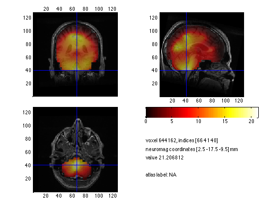
ft_sourceplot(cfg, source_postinterp);
the input is volume data with dimensions [256 256 256]
scaling anatomy to [0 1]
no masking parameter

click left mouse button to reposition the cursor
click and hold right mouse button to update the position while moving the mouse
use the arrowkeys to navigate in the current axis
the call to "ft_sourceplot" took 7 seconds and required the additional allocation of an estimated 433 MB

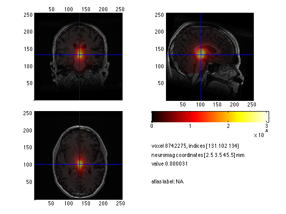
Notice that the estimated power is strongest in the center of the brain.
INSTRUCTION: Discuss why the source power is overestimated in the center of the brain. Hint 1: what are the leadfield values in the center of the head? Why? Hint 2: Remember the 'unit-gain constraint' of beamformer spatial filters.
There are several ways of circumventing the noise bias towards the center of the head which we will show below.
If it is not possible to compare two conditions (e.g. A versus B or post versus pre) one can apply the neural activity index (NAI), in order to remove the center of the head bias shown above. The NAI is the power normalized with an estimate of the spatially inhomogeneous noise. An estimate of the noise has been done by ft_sourceanalysis, by setting cfg.dics.projectnoise='yes' (default is 'no'). This noise estimate was computed on the basis of the smallest eigenvalue of the cross-spectral density matrix. To calculate the NAI do the following:
source_post.avg.nai = source_post.avg.pow ./ source_post.avg.noise;

cfg = [];
cfg.downsample = 2;
cfg.parameter = 'avg.nai';
source_naiinterp = ft_sourceinterpolate(cfg, source_post, mri_resliced);


cfg = [];
cfg.funparameter = 'avg.nai';
ft_sourceplot(cfg, source_naiinterp);
the input is source data with 11340 positions on a [20 27 21] grid
the input is volume data with dimensions [256 256 256]
updating homogenous coordinate transformation matrix
downsampling anatomy
downsampling inside
the call to "ft_volumedownsample" took 0 seconds and required the additional allocation of an estimated 2 MB
selecting subvolume of 20.0%
interpolating
interpolating 95.0%

reslicing and interpolating avg.nai
interpolating
interpolating 95.0%

the call to "ft_sourceinterpolate" took 7 seconds and required the additional allocation of an estimated 23 MB
...
The distribution looks more meaningfull, but still not very clear localized towards the visual region.
Another option, besides contrasting the power to the noise estimate, is to normalize the lead field when you compute it (cfg.normalize='yes' in the call to ft_prepare_leadfield).
INSTRUCTION: Recompute the lead field and source estimate this way and plot the result.
Source Analysis: Contrast activity to another interval
One approach is to compare the post- and pre-stimulus interval, which we describe now. Another approach is to contrast the same window of interest (relative in time to some stimulus or response) between two or more conditions, which we do not show here, but the calls to FieldTrip functions are conceptually the same.
Importantly, if you later want to compare the two conditions statistically, you have to compute the sources based on an inverse filter computed from both conditions, so called 'common filters', and then apply this filter separately to each condition to obtain the source power estimate in each condition separately.
First we concatenate the data, cerating a single data structure with both conditions and compute the frequency domain CSD.
data_all = ft_appenddata([], data_pre, data_post);

cfg = [];
cfg.method = 'mtmfft';
cfg.output = 'powandcsd'; % the CSD is needed for source reconstruction
cfg.taper = 'dpss';
cfg.foi = 50:5:100;
cfg.tapsmofrq = 10;       % we apply plenty of frequency smoothing

freq_all = ft_freqanalysis(cfg, data_all);
input dataset 1, 204 channels, 104 trials
input dataset 2, 204 channels, 101 trials
concatenating the trials over all datasets
the call to "ft_appenddata" took 0 seconds and required the additional allocation of an estimated 1 MB
the input is raw data with 204 channels and 205 trials
processing trials
processing trial 205/205 nfft: 401 samples, datalength: 401 samples, 7 tapers

the call to "ft_freqanalysis" took 35 seconds and required the additional allocation of an estimated 143 MB
Then we compute the inverse spatially adaptive beamformer filter based on both conditions. Note the use of cfg.keepfilter so that the output saves this computed filter.
cfg = [];
cfg.method      = 'dics';
cfg.dics.projectnoise = 'yes'; % also make an estimate of the noise distribution
cfg.dics.lambda       = '5%'; % the data is rank deficient, hence some regularization is needed
cfg.dics.keepfilter   = 'yes';
cfg.frequency   = 90;
cfg.vol         = headmodel;
cfg.grid        = sourcemodel;
source_all = ft_sourceanalysis(cfg, freq_all);
the input is freq data with 204 channels, 11 frequencybins and no timebins
using headmodel specified in the configuration
using gradiometers specified in the data
computing surface normals
creating dipole grid based on user specified dipole positions
using headmodel specified in the configuration
using gradiometers specified in the configuration
5714 dipoles inside, 5626 dipoles outside brain
the call to "ft_prepare_sourcemodel" took 1 seconds and required the additional allocation of an estimated 8 MB
selection crsspctrm along dimension 3
using precomputed leadfields
scanning grid
scanning grid 5714/5714

the call to "ft_sourceanalysis" took 20 seconds and required the additional allocation of an estimated 156 MB
Besides the (now not interesting) source estimate, the source structure contains the spatial filters, i.e. the inverse operator for each position in the dipole grid.
disp(source_all.avg.filter)

disp(source_all.avg.filter{source_all.inside(1)});
    []
    []
    []
    []
    []
    []
    []
    []
    []
    []
    []
    []
    []
    []
    []
...
By placing this pre-computed filter inside cfg.grid.filter, it can now be applied to each condition separately.
cfg = [];
cfg.method      = 'dics';
cfg.frequency   = 80;
cfg.vol         = headmodel;
cfg.grid        = sourcemodel;
cfg.grid.filter = source_all.avg.filter; % pass the precomputed spatial filters

source_precon  = ft_sourceanalysis(cfg, freq_pre );
source_postcon = ft_sourceanalysis(cfg, freq_post);
the input is freq data with 204 channels, 11 frequencybins and no timebins
using headmodel specified in the configuration
using gradiometers specified in the data
computing surface normals
creating dipole grid based on user specified dipole positions
using headmodel specified in the configuration
using gradiometers specified in the configuration
5714 dipoles inside, 5626 dipoles outside brain
the call to "ft_prepare_sourcemodel" took 1 seconds and required the additional allocation of an estimated 73 MB
selection crsspctrm along dimension 3
using precomputed leadfields
using precomputed filters
scanning grid
scanning grid 5714/5714

...
Now we can compute the contrast of post versus pre. In this operation we exploit that the noise bias is the same for the pre- and post-stimulus interval and it will thus be removed.
source_con          = source_postcon;
source_con.avg.pow  = source_postcon.avg.pow ./ source_pre.avg.pow - 1; % center it around 0, i.e. express as relative change
Then we interpolate the source ratio onto the MRI, and plot the result.
cfg = [];
cfg.parameter = 'avg.pow';
source_coninterp = ft_sourceinterpolate(cfg, source_con, mri_resliced);
the input is source data with 11340 positions on a [20 27 21] grid
the input is volume data with dimensions [256 256 256]
selecting subvolume of 20.2%
interpolating
interpolating 95.0%

reslicing and interpolating avg.pow
interpolating
interpolating 95.0%

the call to "ft_sourceinterpolate" took 35 seconds and required the additional allocation of an estimated 0 MB
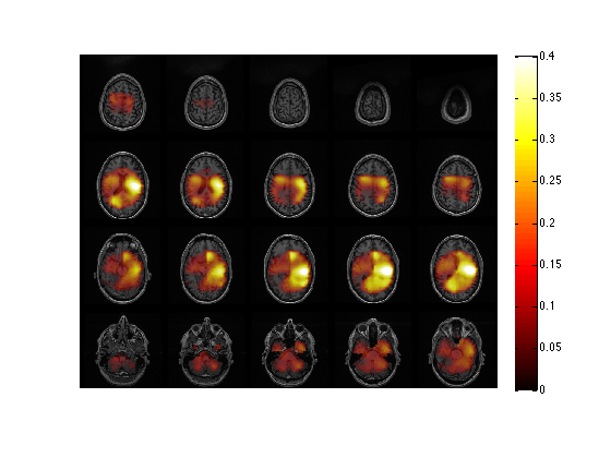
cfg = [];
cfg.method        = 'slice';
cfg.funparameter  = 'avg.pow';
cfg.maskparameter = cfg.funparameter;
cfg.funcolorlim   = [0.0 0.4];
cfg.opacitylim    = [0.0 0.4];
cfg.opacitymap    = 'rampup';
ft_sourceplot(cfg, source_coninterp);
the input is volume data with dimensions [256 256 256]
scaling anatomy to [0 1]
scaling anatomy
the call to "ft_sourceplot" took 5 seconds and required the additional allocation of an estimated 179 MB
The common-filter contrast can be compared to the ratio of the two conditions estimated separately.
source_ratio         = source_post;
source_ratio.avg.pow = source_post.avg.pow ./ source_pre.avg.pow - 1; % center it around 0, i.e. express as relative change

cfg = [];
cfg.parameter = 'avg.pow';
source_ratiointerp = ft_sourceinterpolate(cfg, source_ratio, mri_resliced);
the input is source data with 11340 positions on a [20 27 21] grid
the input is volume data with dimensions [256 256 256]
selecting subvolume of 20.2%
interpolating
interpolating 95.0%

reslicing and interpolating avg.pow
interpolating
interpolating 95.0%

the call to "ft_sourceinterpolate" took 18 seconds and required the additional allocation of an estimated 669 MB
cfg = [];
cfg.method        = 'slice';
cfg.funparameter = 'avg.pow';
cfg.maskparameter = cfg.funparameter;
cfg.funcolorlim   = [0.0 0.2];
cfg.opacitylim    = [0.0 0.2];
cfg.opacitymap    = 'rampup';
figure
ft_sourceplot(cfg, source_ratiointerp);
the input is volume data with dimensions [256 256 256]
scaling anatomy to [0 1]
scaling anatomy
the call to "ft_sourceplot" took 2 seconds and required the additional allocation of an estimated 0 MB

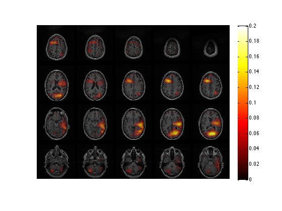
The common-filter approach results in a spatial localization that is less clear than the separate-filter approach. This suggests that the data is very different in the baseline and stimulus condition and that pooling the CSD matrices is not a good way to optimize the spatial selectivity of the beamformer filters and to suppress the noise from uncorrelated (physiological or environmental) sources. Using separate filters for baseline and activation is better in this case. However, if you compare data in two conditions where the experimental manipulation is more subtle, the common filters approach is in general the most appropriate and sensitive.
Now that we have the source reconstruction results, we can plot them in a visually more appealing manner. For this we refer to the original online beamformer tutorial.
Summary and suggested further reading
Beamforming source analysis in the frequency domain with DICS has been demonstrated. An example of how to compute a head model (single shell) and forward lead field was shown. Various options for contrasting the time-frequency window of interest against a control was shown, including against 'noise' (NAI: minimum eigenvalue of the CSD) and against the pre-stimulus window using a 'common filter'. Options at each stage and their influence on the results were discussed, such as lead field normalization and CSD matrix regularization. Finally, options for plotting on slices, orthogonal views, or on the surface were shown.
Details on head models can be found here or here. Computing event-related fields with MNE or LCMV might be of interest. More information on common filters can be found here. If you are doing a group study where you want the grid points to be the same over all subjects, see here. See here for source statistics.